Project Outcomes
- KPIs: Efficiency (η), Specific Power Consumption (SPC), Downtime analysis.
- Type-level benchmarks (75th percentile efficiency) and estimated input kW savings to reach benchmark.
- Predictive maintenance: linear trend on last 90 days; projected threshold crossing at η < 0.72.
- Excel dashboard consolidates charts and sheets for quick review and pivoting.
Input Sources & Methods
- Simulated Dataset: 48 machines × 210 days (Motors, Pumps, Compressors, Turbines).
- Signals: load %, RPM, torque (Nm), temperature (°C), vibration (mm/s), mechanical output (kW), input power (kW), downtime (min).
- Python: Pandas, NumPy, Matplotlib for cleaning, KPIs, charts.
- Excel: Dashboard with charts; pivot-style summaries in TypeSummary; savings & predictive sheets.
Efficiency Distribution by Type
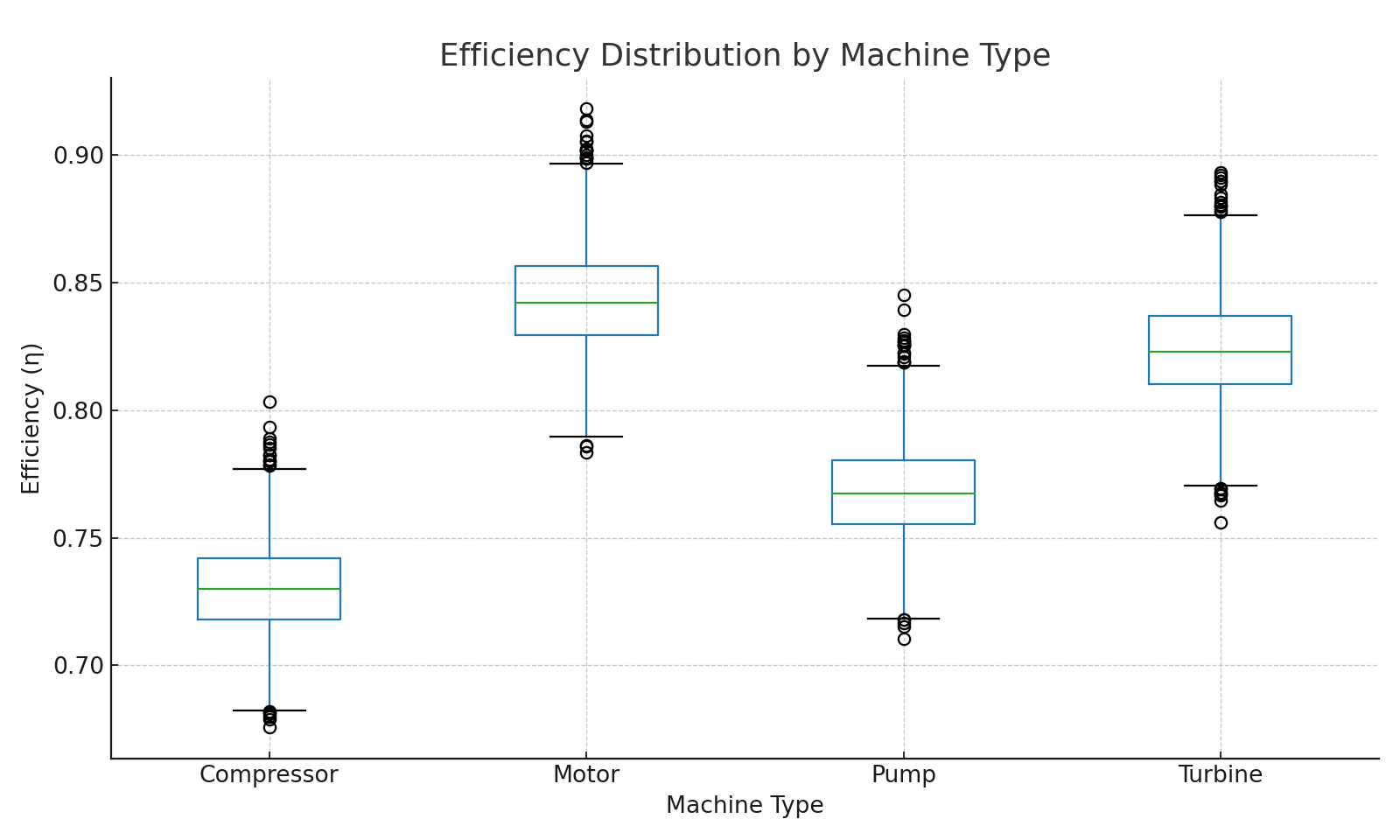
Median and spread of η across Motors, Pumps, Compressors, Turbines.
7‑Day Rolling Efficiency — Worst 4 Machines
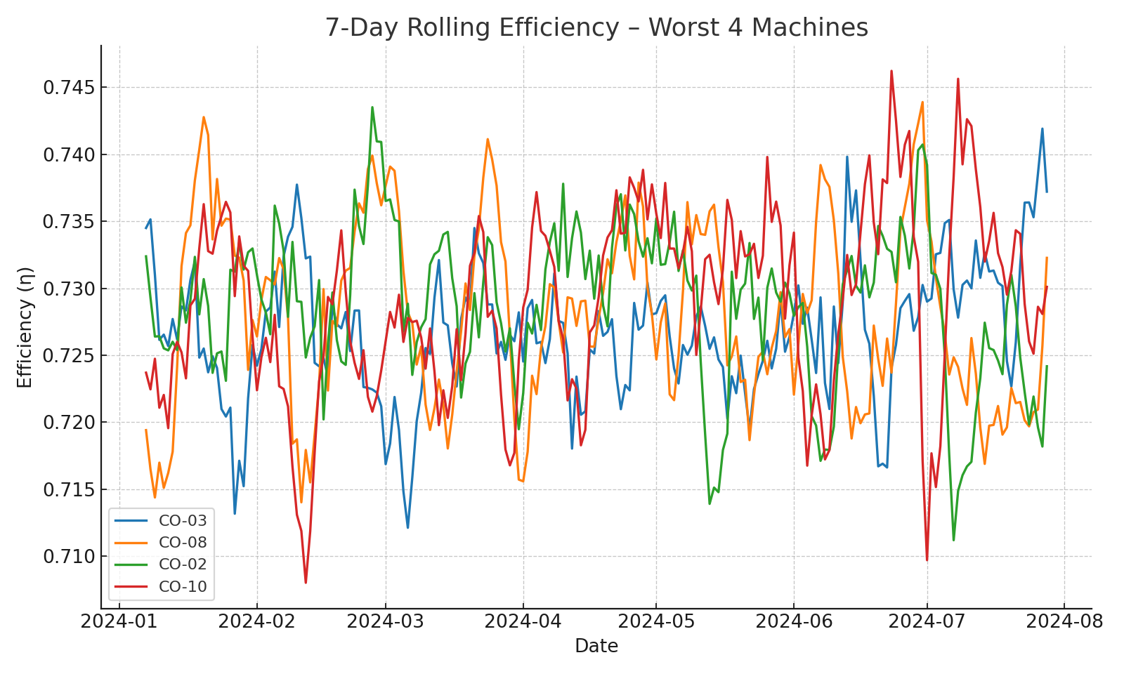
Helps identify persistent underperformers for targeted maintenance.
Temperature vs Vibration
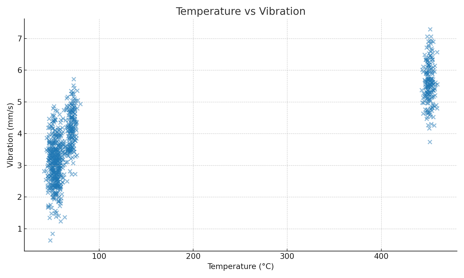
Elevated vibration alongside high temperature often precedes efficiency decay.
Average Specific Power Consumption by Type
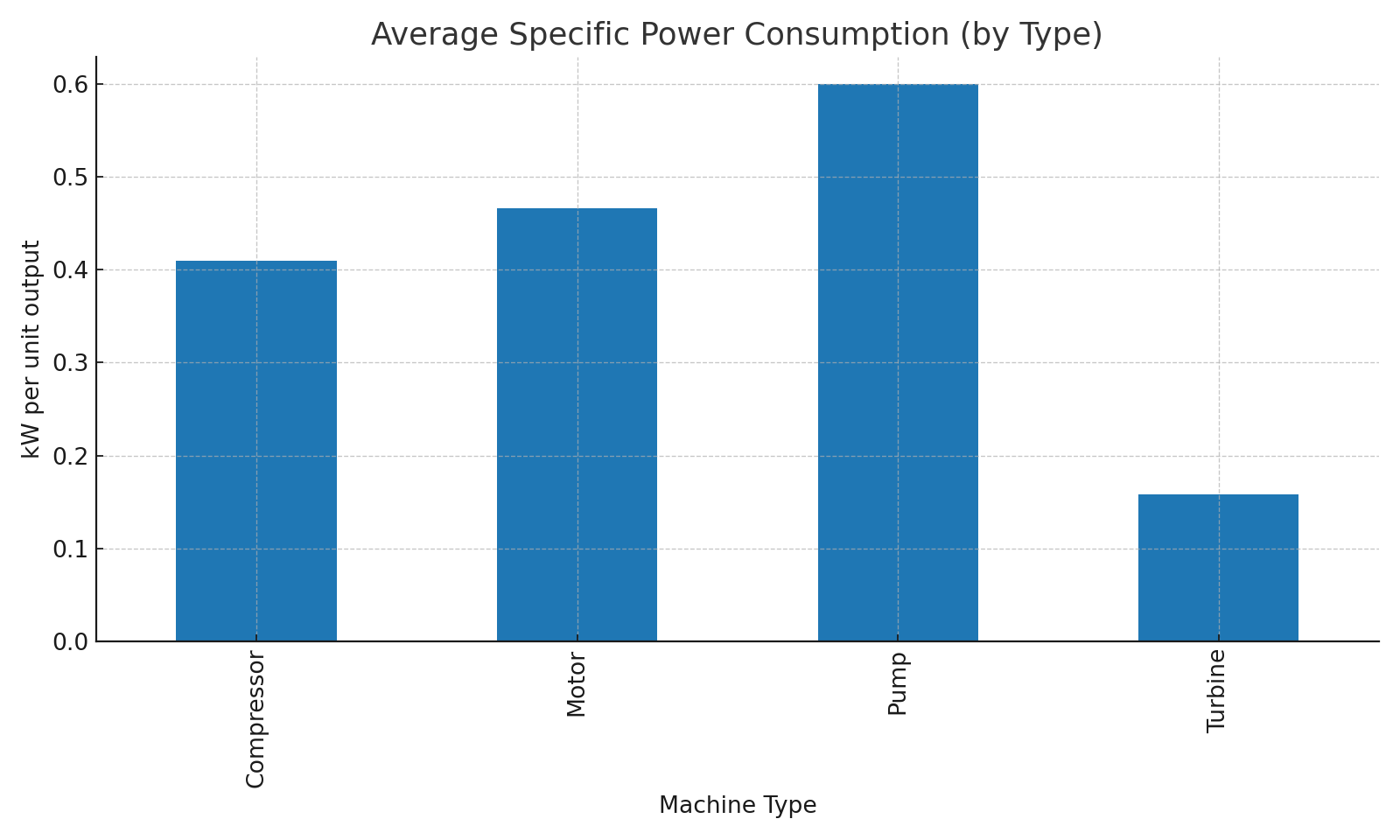
Lower is better; SPC = input kW / unit output.
Type-level Summary (sample)
| type | avg_efficiency | median_efficiency | avg_spc | avg_input_kW | total_downtime_min | eff_benchmark |
|---|---|---|---|---|---|---|
| Compressor | 0.730 | 0.730 | 0.410 | 7.670 | 3560 | 0.742 |
| Motor | 0.843 | 0.842 | 0.467 | 5.164 | 3307 | 0.856 |
| Pump | 0.768 | 0.767 | 0.600 | 6.391 | 3992 | 0.780 |
| Turbine | 0.824 | 0.823 | 0.158 | 5.464 | 3511 | 0.837 |
Top Savings Opportunities (sample)
| machine_id | type | current_efficiency | benchmark_efficiency | potential_input_kW_savings |
|---|---|---|---|---|
| CO-03 | Compressor | 0.727 | 0.742 | 0.161 |
| CO-08 | Compressor | 0.728 | 0.742 | 0.142 |
| CO-10 | Compressor | 0.729 | 0.742 | 0.133 |
| CO-02 | Compressor | 0.729 | 0.742 | 0.131 |
| CO-06 | Compressor | 0.730 | 0.742 | 0.126 |
| PU-08 | Pump | 0.766 | 0.780 | 0.121 |
| CO-05 | Compressor | 0.730 | 0.742 | 0.121 |
| CO-04 | Compressor | 0.730 | 0.742 | 0.117 |
| CO-01 | Compressor | 0.730 | 0.742 | 0.116 |
| PU-09 | Pump | 0.767 | 0.780 | 0.110 |
| CO-11 | Compressor | 0.731 | 0.742 | 0.108 |
| CO-07 | Compressor | 0.731 | 0.742 | 0.107 |
Predictive Maintenance (sample)
| machine_id | current_eff_mean_90d | trend_slope_per_day | predicted_days_to_cross_threshold | predicted_date_below_threshold |
|---|---|---|---|---|
| CO-02 | 0.727 | -0.000 | None | None |
| CO-08 | 0.727 | -0.000 | None | None |
| CO-06 | 0.727 | 0.000 | None | None |
| CO-03 | 0.728 | 0.000 | None | None |
| CO-07 | 0.729 | 0.000 | None | None |
| CO-05 | 0.729 | 0.000 | None | None |
| CO-04 | 0.731 | -0.000 | None | None |
| CO-01 | 0.731 | 0.000 | None | None |
| CO-11 | 0.731 | -0.000 | None | None |
| CO-10 | 0.732 | 0.000 | None | None |
| CO-12 | 0.732 | 0.000 | None | None |
| CO-09 | 0.732 | 0.000 | None | None |
How to Reproduce
- Run the provided Python notebook/script to simulate data, compute KPIs, and export assets.
- Open Energy_Efficiency_Analysis_Dashboard.xlsx → Review “Dashboard” (charts), then explore TypeSummary, SavingsOpportunities, and PredictiveMaintenance.
-
Adjust thresholds (e.g., η threshold =
0.72) or cost per kWh to translate savings into ₹/year. - For Excel What‑If: vary load %, temperature, or vibration to see SPC and η sensitivities.
Formulas
- Efficiency (η) = Mechanical Output kW / Input Power kW
- Specific Power Consumption (SPC) = Input Power kW / Unit Output (per hr)
- Potential Savings (kW) ≈ Output kW × (1/ηcurrent − 1/ηbenchmark)